
GGU-SIEVE -e
Evaluation and presentation of sieve and hydrometer analysis to DIN 18123 and DIN EN ISO 17892-4
GGU-SIEVE
Version 17

Contents:
Preface
The GGU-SIEVE program system allows evaluation and presentation of (combined) sieve and hydrometer analyses according to DIN EN ISO 17892-4:2017-04. The soil type can be determined according to DIN 4022, DIN EN ISO 14688-1 or ASTM.
10 tests can be edited and presented simultaneously by the program. Notes and the results of these ten tests are presented in a table on the output form (diagram table). It is necessary to restrict the table to ten tests for space reasons; more tests will not fit in the table.
Input of further 100 tests is possible with the "Special" menu. For these tests (to be called extra grain size distributions or extra GSDs), no entry in the table is made. Only a legend will be shown, making possible an allocation of line type and test designation. Using the extra GSDs, it is also possible to define boundary curves. Further to this, hatching can be created to enhance the boundary areas.
Data input is in accordance with WINDOWS conventions and can therefore be learned almost without a manual. Graphics output supports the true-type fonts supplied with WINDOWS, so that excellent layout is guaranteed. Colour output and any graphics (e.g. files in formats BMP, JPG, PSP, TIF, etc.) are supported. PDF and DXF files can also be imported by means of the integrated Mini-CAD module (see the "Mini-CAD" manual).
The program has been successfully used in many projects by renowned consultancies and institutes and has been thoroughly tested. The program system has been thoroughly tested. No faults have been found. Nevertheless, liability for completeness and correctness of the program and the manual, and for any damage resulting from incompleteness or incorrectness, cannot be accepted.
Licence protection
To protect the GGU software from unauthorised access, each GGU program is equipped with the CodeMeter software protection system from WIBU-Systems. Each GGU programme is bound to a so-called CmContainer via a licence with the corresponding product code.
We use 3 alternative CmContainer types, which are stored on your PC, the so-called CodeMeter licence server:
CmStick
The licence is stored in a USB dongle.
CmActLicense (soft licence, not for virtual PC/servers)
The licence is stored in a licence file that is bound to the hardware of a computer.
CmCloudContainer
The licence is located on a CmCloud server of WIBU-Systems and is mirrored to your CodeMeter licence server.
For the CodeMeter protection system, the driver software CodeMeter Runtime Kit must be installed on your PC (CodeMeter licence server). The GGU program checks at start-up and during running time whether a licence is present on a CmContainer.
Language selection
GGU-SIEVE is a bilingual program. The program always starts with the language setting applicable when it was last ended.
The language preferences can be changed at any time in the "Info" menu, using the menu item "Spracheinstellung" (for German) or "Language preferences" (for English).
Starting the program
After starting the program, you will see two menus at the top of the window:
File
Info
After clicking the "File" menu, either an existing file can be loaded by means of the "Load" menu item, or new tests can be entered using "New". After clicking "File/New" an empty form is displayed on the screen. Then, the menu bar will show six menus:
File
Edit
Graphics preferences
Output preferences
Special
Info
After clicking one of these menus, the menu items roll down, allowing you access to all program functions.
The program works on the principle of What you see is what you get. This means that the screen presentation represents, overall, what you will see on your printer. In the last consequence, this would mean that the screen presentation would have to be refreshed after every alteration you make. For reasons of efficiency and as this can take several seconds for complex screen contents, the GGU-SIEVE screen is not refreshed after every alteration.
If you would like to refresh the screen contents, press either [F2] or [Esc]. The [Esc] key additionally sets the screen presentation back to your current zoom, which has the default value 1.5, corresponding to an A4 sheet in landscape format.
Tips and tricks
Keyboard and mouse
If you click the right mouse button anywhere on the screen a context menu containing the principal menu items opens.
By double-clicking the left mouse button on output sheet elements or Mini-CAD objects, the editor for the selected object immediately opens, allowing it to be edited. By double-clicking output sheet elements while holding the [Shift] key, the preferences for the position, size and appearance of the element open for editing in the editor.
In most dialog boxes, the buttons for leaving the box or buttons for decisive functions are marked thickly and can be reached by clicking the [Enter]/[Return] key.
In dialog boxes in which you have to make entries, the quickest way to jump to the next input box is to use the [Tab] key. The previous value is marked and can be overwritten directly with the new entry. You do not have to move to the box with the mouse and delete the old entry in advance.
In input boxes for numerical values, you can also use common arithmetic operations to adjust (see Section 5.2).
You can scroll the screen with the keyboard using the cursor keys and the [Page up] and [Page down] keys. After activating the zoom functions, click on an area of the screen to enlarge or reduce the display by a factor of 2. Alternatively, by clicking and dragging the mouse while holding down the [Ctrl] key, you define a window section which is then displayed in full screen.
You can also use the mouse wheel to zoom in or out or to move the screen display. For mouse wheel operation, the setting according to Windows conventions is activated by default:
Mouse wheel up = move screen image up
Mouse wheel down = move screen image down
[Shift] + mouse wheel up = move screen image right
[Shift] + mouse wheel down = move screen image left
[Ctrl] + mouse wheel up = enlarge screen image (zoom in)
[Ctrl] + mouse wheel down = shrink screen image (zoom out)
From a zoomed representation you return to the full screen with [Esc].
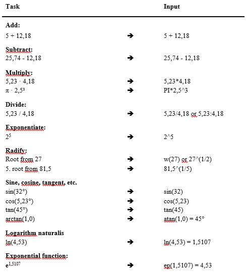
Calculation operations in input boxes with numbers
In input boxes for numerical values, you can use the following calculation operations, also in
combinations, to determine the desired value or to adjust the existing value. After pressing the [Return] or [Enter] key, the determined value is inserted.
Function keys
Some of the function keys are assigned program functions. The allocations are noted after the corresponding menu items. The individual function key allocations are:
[Esc] refreshes the screen contents and sets the screen back to the given format (A4 landscape). This is useful if, for example, you have used the zoom function to display parts of the screen and would like to quickly return to a complete overview.
[F1] opens the manual file.
[F2] refreshes the screen without altering the current magnification.
[F11] activates the menu item "Output preferences/Move objects".
File extensions
In the GGU-SIEVE program, you can save or open files containing certain settings and data at a number of points. Files marked by * are always opened when the program starts if they are saved at the program level using the name GGU-SIEVE.
.kvs All input, settings and Mini-CAD objects
-> "File/Save"/"File/Load"
.ekv The sieving and/or hydrometer analysis data of an individual grain size distribution
-> "Edit/Grain size distribution" -> Button with GSD no. -> Grain size distribution editor
-> Buttons "Load GSD"/"Save GSD"
.aer* Hydrometer data for a variety of hydrometers
-> "Edit/Grain size distribution" -> Button with GSD no. -> Grain size distribution editor
-> Button "Hydrometer values" -> Buttons "Load"/"Save"
.scä* Time and temperature specifications for a hydrometer analysis
-> "Edit/Grain size distribution" -> Button with GSD no. -> Grain size distribution editor
-> Button "Edit hydrometer analysis data" -> Buttons "Load"/"Save"
.sbe* Sieve combination (activated sieves and their diameters)
-> "Edit/Grain size distribution" -> Button with GSD no. -> Grain size distribution editor
-> Button "Edit sieving data" -> Buttons "Load"/"Save"
.stf* Grain size distribution pen settings
"GGU-SIEVE.stf": Diagram table grain size distributions
-> "Graphics preferences/Pen colour and width" -> Buttons "Load"/"Save"
"EXTRAKVS.stf": Extra grain size distributions in the menu "Special"
-> "Special/Extra GSDs preferences" -> Button "Extra GSDs pens"
-> Buttons "Load"/"Save"
.alg* Preferences under "Graphics preferences/Preferences" and
menu items in menu "Output preferences"
-> "Graphics preferences/Load graphics preferences"/"Graphics preferences/Save graphics preferences"
.ktx Texts and allocations for diagram table
-> "Output preferences/Texts + table" "Diagram table" group box
-> Button "Edit texts and allocation" -> Buttons "Load"/"Save"
.xkv All extra grain size distributions entered in the "Special" menu with the
associated preferences for hatching and pens
-> "Special/Load extra GSDs"/ Special/Save extra GSDs"
"Copy/print area" icon
A dialog box opens when the "Copy/print area" icon in the menu toolbar is clicked,
describing the options available for this function. For example, using this icon it is possible to either copy areas of the screen graphics and paste them into the report, or send them directly to a printer.

In the dialog box, first select where the copied area should be transferred to: "Clipboard",
"File" or "Printer". The cursor is displayed as a cross after leaving the dialog box and, keeping the left mouse button pressed, the required area may be enclosed. If the marked area does not suit your requirements, abort the subsequent boxes and restart the function by clicking the icon again.
If "Clipboard" was selected, move to the MS Word document (for example) after marking the area and paste the copied graphics using "Edit/Paste". If "File" was selected, the following dialog box opens once the area has been defined:
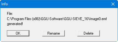
The default location of the file is the folder from which the program is started and, if several files are created, the file is given the file name "Image0.emf" with sequential numbering. If the
"Rename" button in the dialog box is clicked, a file selector box opens and the copied area can be saved under a different name in a user-defined folder. Saving can be aborted by pressing the "Delete" button.
If the "Printer" button was pressed in the first dialog box, a dialog box for defining the printer settings opens after marking the area. Following this, a dialog box for defining the image output settings opens. After confirming the settings the defined area is output to the selected printer.
Description of menu items
File menu
"New" menu item
All data entered are deleted after a confirmation prompt. New tests can then be entered.
"Load" menu item
You can load a file with test data, which was created and saved at a previous sitting, and then edit the test data.
"Add file" menu item
Using this menu item it is possible to load the results of a number of tests, stored on disk as separate files, in order to visualise them together on one sheet. The tests contained in the added file will be appended to the current record.
Please note that the information concerning the page format, general entries (e.g. company name, project description, report no.) and preferences (e.g. grading curve pens) are not imported with the appended file.
Any annotations or settings should therefore be defined after appending or be present in the last opened file.
"Save" menu item
You can save data entered or edited during program use to a file, in order to have them available at a later date, or to archive them. The data is saved without prompting with the name of the current file. Loading again later creates exactly the same presentation as was present at the time of saving.
"Save as" menu item
You can save data entered during program use to an existing file or to a new file, i.e. using a new file name. For reasons of clarity, it makes sense to use ".kvs" as file suffix, as this is the suffix used in the file requester box for the menu item "File/Load". If you choose not to enter an extension when saving, ".kvs" will be used automatically.
"Print 'simple' output table" menu item
A result table containing the results of all current tests can be printed or saved in a file (e.g. for further editing in a word processing application ). Output consists of a type of laboratory protocol of all sieve and hydrometer analyses, as entered in the menu item "Edit/Grain size distribution". By going to the menu item "Graphics preferences/View output table" (see Section 6.3.1) you can view and print the laboratory output table for individual tests in the shape of a submission quality output sheet.
After going to this menu item, you can decide whether the special data (e.g. the diameter of certain percentage passages, derived quantities such as k or the coefficient of curvature, grain fraction percentages, etc.) are also printed.
You will then see the following dialog box for specifying output preferences.
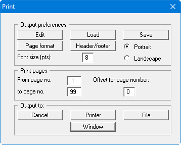
"Output preferences" group box
Using the "Edit" button the current output preferences can be changed or a different printer selected. Using the "Save" button, all preferences from this dialog box can be saved to a file in order to have them available for a later session. If you select "GGU-SIEVE.drk" as file name and save the file in the program folder (default), the file will be automatically loaded the next time you start the program.
Using the "Page format" button you can define, amongst other things, the size of the left margin and the number of lines per page. The "Header/footer" button allows you to enter a header and footer text for each page. If the "#" symbol appears within the text, the current page number will be entered during printing (e.g. "Page #"). The text size is given in "Pts". You can also change between "Portrait" and "Landscape" formats.
"Print pages" group box
If you do not wish pagination to begin with "1" you can add an offset number to the check box. This offset will be added to the current page number. The output range is defined using "From page no." "to page no.".
"Output to:" group box
Start direct log output by clicking the "Printer" button. Start output to an ".erg" result file by pressing the "File" button. The file name can then be selected from or entered into the box. If the "Window" button is selected the results are sent to a new window and can be edited there at will. Using this window's menu the edited logs can be saved to a ".txt" text file or printed or an existing text file be opened.
"Save XMLfile" menu item
As with the previous menu item, you can output a results log of all tests, but in this case as an XML file.
"Output preferences" menu item
You can edit output preferences (e.g. swap between portrait and landscape) or change the printer in accordance with WINDOWS conventions.
"Print and export" menu item
You can select your output format in a dialog box. You have the following possibilities:
"Printer"
allows graphic output of the current screen contents. to the WINDOWS standard printer
or to any other printer selected using the menu item "File/Output preferences". But
you may also select a different printer in the following dialog box by pressing the
"Output prefs./change printer" button.
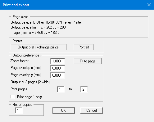
In the upper group box, the maximum dimensions which the printer can accept are given. Below this, the dimensions of the image to be printed are given. If the image is larger than the output format of the printer, the image will be printed to several pages (in the above example, 2). In order to facilitate better re-connection of the images, the possibility of entering an overlap for each page, in x and y direction, is given. Alternatively, you also have the possibility of selecting a smaller zoom factor, ensuring output to one page ("Fit to page" button). Following this, you can enlarge to the original format on a copying machine, to ensure true scaling. Furthermore, you may enter the number of copies to be printed.
"DXF file"
allows output of the graphics to a DXF file. DXF is a common file format for transferring graphics between a variety of applications.
"GGU-CAD file"
allows output of the graphics to a file, to enable further processing with the
GGU-CAD program. Compared to output as a DXF file this has the advantage that no
loss of colour quality occurs during export.
"Clipboard"
The graphics are copied to the WINDOWS clipboard. From there, they can be imported into other WINDOWS programs for further processing, e.g. into a word processor. In order to import into any other WINDOWS program you must generally use the "Edit/Paste" function of the respective application.
"Metafile"
allows output of the graphics to a file to be further processed with third party software. Output is in the standardised EMF format (Enhanced Metafile format). Use of the Metafile format guarantees the best possible quality when transferring graphics.
If you select the "Copy/print area" tool from the toolbar, you can copy parts of the graphics to the clipboard or save them to an EMF file. Alternatively, you can send the marked area directly to your printer (see "Tips and tricks", Section 5.5).
Using the "Mini-CAD" program module you can also import EMF files generated using other GGU applications into your graphics.

"Mini-CAD"
allows export of the graphics to a file to enable importing to different GGU applications with the Mini-CAD module.
"GGUMiniCAD"
allows export of the graphics to a file to enable processing in the GGUMiniCAD program.
"Cancel"
Printing is cancelled.
"Batch print" menu item
If you would like to print several appendices at once, select this menu item. You will see the following dialog box:
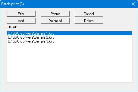
Create a list of files for printing using "Add" and selecting the desired files. The number of files is displayed in the dialog box header. Using "Delete" you can mark and delete selected individual files from the list. After selecting the "Delete all" button, you can compile a new list. Selection of the desired printer and output preferences is achieved by pressing the "Printer" button.
You then start printing by using the "Print" button. In the dialog box which then appears you can select further preferences for printer output such as, e.g., the number of copies. These preferences will be applied to all files in the list.
"Exit" menu item
After a confirmation prompt, you can quit the program.
"1, 2, 3, 4" menu items
The "1, 2, 3, 4" menu items show the last four files worked on. By selecting one of these menu items the listed file will be loaded. If you have saved files in any other folder than the program folder, you can save yourself the occasionally onerous rummaging through various sub-folders.
Edit menu
"Sieving weight preferences" menu item
The sieving residue determined for a sieve analysis can be entered as a cumulative weight. This function is deactivated by default. If the check box "Sieving input via summed weights" is activated later, the residues entered for the individual sieves are added for existing sieve analyses.
If you are working with partial sieving, you can activate "Partial sieving according to DIN EN 933-1" here. When entering the sieving data, you will then receive an extended input box for partial sieving.
"Grain size distribution" menu item
Central data input
This point represents the program's central menu item. Almost all the sieving and/or hydrometer test data are entered here. As an example, after clicking this menu item the following dialog box opens:
Three tests are already present in this example. The tests are automatically numbered and the test numbers ("1, 2, 3, ...") shown on the respective buttons. The following actions are possible:
"To menu bar"
You return to the original menu bar.
"New"
You can now enter data for a new test.
"1", "2", ...
By clicking the buttons labelled with the test numbers you can open and edit the data for the corresponding test.
Presentation of the grading curves and the corresponding columns or rows in the diagram table always follows the sequence of the test numbers.
The presentation sequence can be altered by going to "Edit/Swap GSDs" (see Section 6.2.4). The selected tests are then assigned the specified new test numbers.
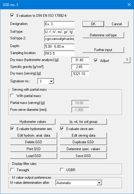
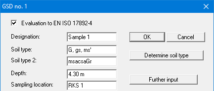
After clicking on "New" or on the button of an existing test a dialog box opens for entering the test data. You can access the editor quickly by double-clicking in the table region containing the required grading curve.
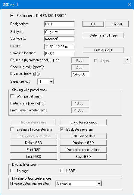
The input boxes and command boxes marked in red in the following dialog box must be filled in or selected regardless of the type of test. The unmarked command boxes and input boxes in the following dialog box are activated or filled in dependent on the test type. They are therefore described in the following sections in accordance with the test type (see Sections 6.2.2.2 to 6.2.2.5).
The texts in the input boxes in the upper marked region can, if required, be shown in the table on the output form (see Section 6.4.2.2 "Output preferences/Texts + table" menu item, button
"Edit texts and allocations").
The following input or actions can be carried out regardless of the type of test:
"Evaluation to EN ISO 17892-4"
If the check box is activated, input and evaluation are compliant with EN ISO 17892-4.
"OK"/"Cancel"
You exit the dialog box. Any changes made are accepted using the "OK" and rejected using the "Cancel" button.
"Designation"
You can enter any designation for the test. If it is a newly created test, the program initially awards the next test number in sequence. For example, if two tests already exist the next new test is given the designation "3". If the designation is to be displayed on the test buttons, deactivate the "Editor with GSD no." check box in the "Graphics preferences/ Preferences" menu item (see Section 6.3.2).
"Soil type"/"Soil type 2"
You can enter the soil type by hand or edit the soil type determined by the program, e.g. by entering U, s in place of U, gs', ms', fs'.
"Determine soil type"
After entering your test data two soil types can be determined by the program in accordance with the user-selected standard by pressing this button (see Section 6.4.2.3). The soil types are automatically included in the "Soil type" and "Soil type 2" input boxes and subsequently entered in the diagram table (see Section 6.4.2.2, "Diagram table" group box).
The overline shown on accessory soil types with a constituent proportion of more than 30-45% (e.g. soil type: very silty) is affected by entering "@" in front of the letter to be overlined.
The "@u" character string in the "Soil type" input box is thus displayed on the form on the screen and in print as "ū".
"Depth"
You can enter information on the depth from which your sample was taken. The unit must also be entered as text.
"Sampling location"
You can enter a more detailed description of the sampling point, e.g. Sampling point 1.
"Signature no.:"
If you want to assign a specific signature to each grain size distribution, you can choose between 10 signatures. The selection menu is only displayed if you have previously deactivated the "Assign signature automatically" check box in the "Graphics preferences/Preferences" menu item (see Section 6.3.2, page 39).
"Further input"
You will see this button for entering additional texts only if the "Free text" option was
used when defining the texts in the diagram table using the menu item "Output preferences/Texts + Table", "Edit texts and allocations" button (see Section 6.4.2.2, page 46).
"Ip, wL for soil groups"
The program identifies the soil groups to DIN 18196 from the given test data if this function has been activated in "Output preferences/Texts + Table", "Edit texts and allocations" button (see Section 6.4.2.2).
The coefficient of plasticity IP and the liquid limit wL must be provided for cohesive soils in order to identify the soil group to DIN 18196 (see the following dialog box). Otherwise, nothing will be displayed in the diagram table on the output form.

You can achieve visualisation of the DIN 18196 soil group for a filled soil, e.g. [GW], if the "Soil is filled" check box is activated.
"Delete GSD"
After a confirmation prompt the currently displayed test is deleted.
"Duplicate GSD"
The currently displayed test is duplicated. You are automatically relocated to the next test (= new test designation). All the data used in the old test are transferred to the new one and can be edited.
"Print GSD"
The current test's data can be output as a laboratory log. If the "Normal" button is selected in the opened dialog box, proceed as described in the "File/Print 'simple' output table" menu item (see Section 6.1.6). After clicking the "ASCII" button the current test's data are saved in a ".txt" file. This may then be edited in a word processor, for example.
You can print the data for the current test as a laboratory output table or save it as a file. Further details on output can be taken from.
"Determine spec. values"
Special values (grain diameters for given percentages, uniformity coefficient, kf, etc.) are calculated for the current test and displayed on the screen in message boxes.
"Load GSD" and "Save GSD"
You can save the data for the current grading curve in a separate file with the extension "*.ekv" or load a previously saved grading curve. All the input data in the above "Grain size distribution" dialog box are included in the file and the test data for the hydrometer and/or sieving tests.
If you choose to "Load GSD", the data for the test being currently edited will be overwritten.
If you would like to add a further test using "Load GSD", you must therefore first create a new test using the "New" button in "Edit/Grain size distribution" and then click "Load GSD".
"Display filter rules" group box "Terzaghi" and "USBR"
By selecting these boxes it is possible to display the Terzaghi and USBR (United States Bureau of Reclamation) filter rules for the current grading curve.
"kf value output preferences" group box
If you have activated the "kf value determination via "Edit/Grain size distribution"" check box in the "Output preferences/Texts + table" menu item "Edit texts and allocation" button (see Section 6.4.2.2, page 47), you can define the kf value determination method separately for each grain size distribution. The "Automatic" setting is helpful, as the program then searches for the appropriate method.
Sieve analysis input
For a sieve analysis activate the "Evaluate sieve arm" check box in the dialog box. The relevant input boxes are then activated accordingly.
"Dry mass (sieving) [g]"
Enter the dry mass of the sample in [g].
"Evaluate sieve arm"
Sieving data can only be entered and evaluated if this check box is activated.
"Edit sieve data"
If you press this button you will arrive at the following dialog box, allowing you to enter sieve test data:
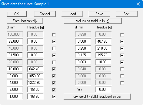
All sieves are initially activated for a new grading curve, i.e. all possible ticks are applied to the third column. Adapt the predefined sieve diameters in the "d [mm]" column to suit the sieve diameters used. Unused sieves, or those without residue, can be removed from the sieve set by unticking the boxes.
To ensure that the grading curve does not end in the graphics at the final value, but instead is displayed up to 100%, the next-larger sieve following the last sieve containing residue should always be additionally activated.
After adapting the sieve diameters, the sieve residues for the individual sieves are entered corresponding to the test data. Press the "(dry weight - SUM residues) as pan" button to calculate the pan residue. The following box is displayed:

The changes are accepted after pressing "OK". If you would prefer to keep the manually entered value, exit the box by pressing "Do not use".
It is generally useful to have the program calculate the pan, because input errors are more easily recognised.
Using the "Enter horizontally"/"Enter vertically" change-over switch dictates horizontal or vertical progress when pressing [TAB]. It is generally useful to enter vertically if only the test data is to be edited. However, you can also navigate these input boxes using the cursor keys [Arrow left], [Arrow right], [Arrow up] and [Arrow down].
If you already have a grading curve (e.g. from a different report) and would like to visualise it using the GGU-SIEVE program, it is much simpler if only the percentages are given for certain diameters. To facilitate this, click the "Values as residue in [g]" in the above dialog box. The text changes to "Values as sum of % finer". All numerical input following the sieve diameters are now entered as sum of the passage in percent. The input value for "Dry mass (sieving) [mm]" is therefore irrelevant. It must only be greater than 0.0.
You can save a special sieve set using "Save". It is thus possible to create separate files for sieve combinations for different purposes. Depending on the test carried out you can open the corresponding sieve set using the "Load" button. If you use the file name "GGU-SIEVE.sbe" for a sieve set and save this file in the program folder, it will be automatically opened when the program starts. The sieves are automatically put into the correct size sequence by pressing the "Sort" button.
Sieving input with partial masses
If you need to sieve large quantities due to the coarseness of the material, it is possible to sieve a partial mass from a smaller sieve diameter. In the example in the following dialog box only 300 g are sieved on the 4 mm sieve, from an original mass of more than 5 kg.
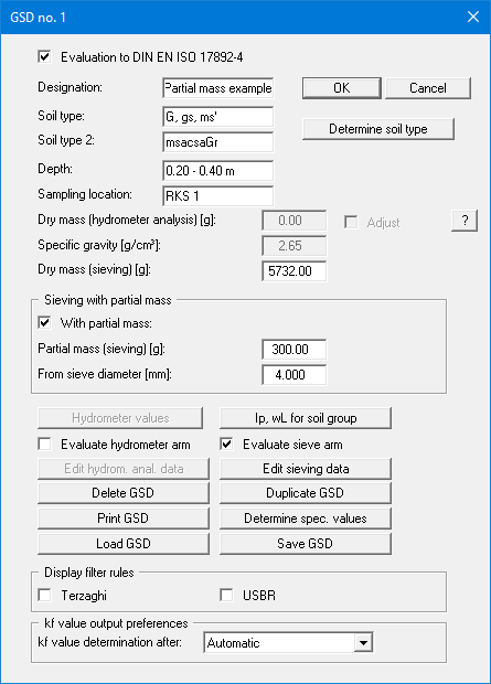
Activate the "With partial mass (sieving) [g]" check box and enter the partial mass in [g] in the following input box; in the example above 300 g. Enter the sieve diameter starting at which the partial mass was sieved in the input box below this; in the example above this is the 4 mm sieve diameter.
Click the "Edit sieve data" button and enter the residues on the large sieves in the dialog box and the partial sieving residues for the 4 mm and smaller sieves. Press the "(Dry weight - SUM residues) as pan" button to calculate the pan weight for the partial sieving.
If you would like to have both the output table sheets output and the graphical visualisation of the grading curve, the residues determined by way of weighing the partial sums are marked in the table by an asterisk ' * '.

Of the original total weight of 5732 g, only 3709.04 g remain after sieve 8.0. Only 300 g of this residual mass is sieved further. The 103.62 g residue determined on sieve 4.0 corresponds to 1281.1 g relative to the residual mass of 3709.04 g. And these 1281.1 g correspond to a percentage residue of 22.35% relative to the total mass of 5732 g.
Hydrometer analysis input
For a pure hydrometer analysis (sedimentation), activate the "Evaluate hydrometer arm" check box in the dialog box. The relevant input boxes are then activated accordingly.

"Dry mass (hydrometer analysis) [g]"
Enter the dry mass of the sample in [g].
"Specific gravity"
Enter the specific gravity of your sample in [g/cm³].
"Hydrometer values"
A dialog box opens for entering the data for the hydrometer used in the test.

Two correction factors are determined when calibrating the hydrometer according to the instructions in EN ISO 17892-4, the meniscus corrections Cm, and R'0. The program automatically corrects the reading values R'h using the factors given above.
If you have made any changes and would like to restore the DIN hydrometer values, press the "Set to DIN hydrometer" button. The current values can be stored in a file using the "Save" button. If you use "GGU-SIEVE.aer" as the file name and save the file in the program folder, the hydrometer values will be active at the next program start. Previously stored hydrometer values can be opened again using "Load".
If you wish to continue evaluation using the DIN 18123 hydrometer method, you can switch back and forth using the lower check box or deactivate the "Evaluation to EN ISO 17892-4" check box in the previous hydrometer analysis editor box (see Section 6.2.2.4).
"Evaluate hydrometer arm"
Hydrometer analysis data can only be entered and evaluated if this check box is activated.
"Edit hydrometer analysis data"
If you press this button you will arrive at the following dialog box, allowing you to enter hydrometer analysis data:
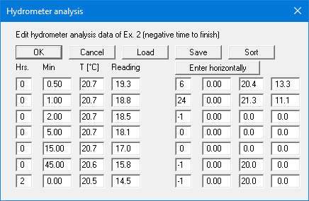
In this box you enter the time of measurement after starting the test in hours and minutes as well as the corresponding temperature. If readings have been taken in second intervals they must be converted to and entered in decimal minutes, i.e. 15 seconds = 0.25 minutes, 30 seconds = 0.5 minutes, etc.
In addition, the uncorrected hydrometer reading R'h is entered in accordance with EN ISO 17892-4, Section 5.3.1.5, i.e. for a reading of 1,0300, 30.0 is entered. The program automatically calculates the corrected reading value using the correction factors you entered.
If the same reading intervals are used every time, the sequence can be stored in a file using "Save". This file can be opened again using "Load". If a sequence is saved with the name "GGU-SIEVE.scä" in the program folder, the file is loaded automatically when the program is started. The times are automatically put into the correct time sequence by pressing the "Sort" button.
Using the "Enter horizontally"/"Enter vertically" change-over switch dictates horizontal or vertical progress when pressing [TAB]. It is generally useful to enter vertically if only the reading data is to be edited. However, you can also navigate these input boxes using the cursor keys [Arrow left], [Arrow right], [Arrow up] and [Arrow down]. Negative time input signals the end of the table.
Combined sieve and hydrometer analysis input
If, because of the quality of the sample, the grain size distribution was determined by sieving and by sedimentation, both the "Evaluate hydrometer arm" and the "Evaluate sieve arm" check boxes must be activated in the "Edit/Grain size distribution" dialog box.

Test value input for the combined sieve/hydrometer analysis is as described in the previous sections dealing with the input for sieving (6.2.2.2) and hydrometer analyses (6.2.2.4). However, when entering dry weights, it should be noted that the program takes the pan weight as a percentage from sieving into consideration for evaluating the hydrometer data. If you perform a sieve and hydrometer analysis using different sample quantities, the "Adjust" check box must be activated. For input of the dry mass then:
Sieving after sedimentation:
The coarse component > 0.125 mm is sieved after sedimentation.
Dry mass (hydrometer analysis) [g] = Total dry mass of sample
Dry mass (sieving) [g] = Total dry mass of sample
The program determines the percentage hydrometer analysis component automatically from the pan weight given for sieving.
Sieving before sedimentation:
The coarse component > 0.125 mm is sieved before sedimentation.
1. Input when testing with one sample:
The entire fines from the tray are adopted for sedimentation.
Dry mass (hydrometer analysis) [g] = Total dry mass of sample
Dry mass (sieving) [g] = Total dry mass of sample
2. Input when testing with two separate samples:
Dry mass (hydrometer analysis) [g] = Total dry mass of the sample used for the
hydrometer analysis
Dry mass (sieving) [g] = Total dry mass of the sample used for sieving
The "Adjust" check box must be activated. The program converts the mass used for hydrometer analysis to the percentage fines from sieving.
"Individual soil type" menu item
Normally, the soil type is determined automatically for every test entered. The default setting for the "Automatic soil type" check box in the dialog box below is therefore activated.
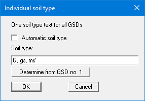
If this check box is deactivated, the soil type rows for the individual grading curves in the diagram table are amalgamated and the soil type entered in the dialog box input is used for all grading curves. The soil type can also be entered by the program by pressing the "Determine from GSD no. 1" button.
"Swap GSDs" menu item
Important grading curve data (e.g. sampling point, depth) are displayed in the table below the diagram. For several grading curves, the presentation sequence corresponds to the input sequence, from left to right. If you would like to change this sequence, you can do so after selecting this menu item.
"Edit GSDs graphically" menu item
After selecting this menu item, you will see information on the functions and can select the curve to be edited. With this function you can move individual points on the curve.
"Edit all GSDs" menu item
Using this menu item, you can delete several existing grain size distributions in one step or adapt the hydrometers for all existing grain distributions.
"Mix GSDs" menu item
A new curve can be created from existing grading curves, mixed from specified proportions of the existing curves. However, at least two pure sieving tests with identical sieve sets must have been entered. You will see the following dialog box:

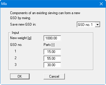
You must first select the test in which the data for the new, mixed grading curve will be saved. Click on "New" if the original grading curves are to be retained. The program then automatically creates a new test. If 10 tests already exist, one of these must be selected in order to save the mixed grading curve.
Enter a weight for the new grading curve in the mixing dialog box above. This will be adopted as the "Dry mass (sieving)". Below this, the proportions of the original grading curves are entered. Portions of grain size distribution curves not to be included in the mix (GSD no. 3 in the example above) are set to zero.
The program identifies the mixed grain fractions and enters them in the sieving data for the selected GSD. To further edit the mixed GSD, click the menu item "Edit/Grain size distribution" and then the corresponding test button or double-click directly in the table area containing the required grading curve.
"Suffosion" menu item
You can choose between two methods:
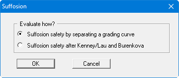
Suffosion safety by separating a grading curve
For verification of suffosion safety in accordance with the Merkblatt Anwendung von Kornfiltern an Bundeswasserstraßen (MAK) (Fact Sheet for the Application of Grain Filters on Waterways), published by the Bundesanstalt für Wasserbau (BAW) in Karlsruhe (2013), it is necessary to divide the grading curves into 2 new curves at a given grain diameter.
In this menu item's dialog box, select the grading curve to be divided and specify the passage or grain size at which it is to be separated.
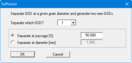
The program now displays a message box with the grain diameter or the %. passage If you adopt the values, the selected grading curve is separated. A further message box is then displayed with information on the passages of the new grain size distribution. This can be copied directly into the clipboard. After closing the box, the two new grain size distributions are displayed in the graphics.
The suffosion safety of these soils can then be examined via an analysis of the filter stability after Cistin/Ziems (see Section 6.2.9.1).
Suffosion safety after Kenney/Lau and Burenkova
This method is described in the Merkblatt Materialtransport im Boden (MMB) (Fact Sheet Material Transport in the Soil) published by Bundesanstalt für Wasserbau (BAW) in Karlsruhe (2013). Here, too, you must first decide which grading curve to evaluate. You are then presented with a message box containing the determined parameters.
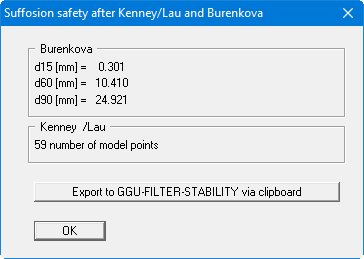
After clicking the export button the program first offers advice on the procedure for using the data copied to the clipboard in the GGU-FILTER-STABILITY program. After confirming the message text, the data are copied to the Windows clipboard and you return to the menu bar.
"Filter stability" menu item
This menu item provides you with two export options for transferring the soil parameters to the GGU-FILTER-STABILITY program:
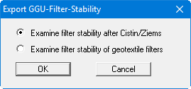
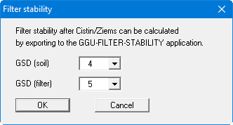
Examine filter stability after Cistin/Ziems
To examine the necessity of a filter layer in accordance with the Merkblatt Anwendung von Kornfiltern an Bundeswasserstraßen (MAK) (Fact Sheet for the Application of Grain Filters on Waterways), published by the Bundesanstalt für Wasserbau (BAW) in Karlsruhe, 2013 (Annex 2), the necessary soil properties (uniformity coefficients U and passage d50) can be determined from existing grain size distribution curves for the relevant soils using this menu item. To do this, select the grain size distributions representing the soil and the filter from the dialog box.
The program then displays the determined values in a message box. The data can be transferred to the GGU-FILTER-STABILITY program via the Windows clipboard using the appropriate button.
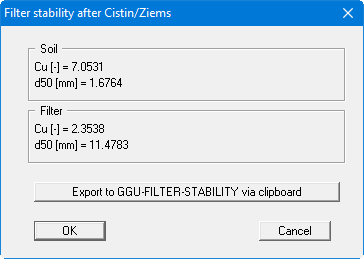
After clicking the export button, the program first offers advice on the procedure for using the data copied to the clipboard in the GGU-FILTER-STABILITY program. After confirming the text the original dialog box opens again allowing the relevant grain size distributions to be selected. Exit the dialog box above by pressing "Cancel".
Examine filter stability of geotextile filters
With regard to examining the filter stability of geotextile filters to Fact Sheet DWA-M 511 use this menu item to determine the necessary soil properties (grain size at d50 and uniformity coefficient Cu) from the grading curve of the relevant soil, which is selected in a dialog box if several grain size distributions are present.

The program then displays the determined values in a message box.

The data can be copied to the Windows clipboard in the usual way using the button "Export to GGU-FILTER-STABILITY via clipboard". If no additional grading curves need to be examined, exit the dialog box by clicking the "Cancel" button.
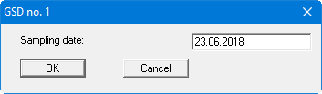
"General" menu item
Go to this menu item to enter general data such as the project identification, report number, annex number, sampling date, etc. This data is displayed in the correct elements of the output sheet.
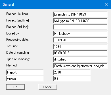
The marked texts in the dialog box also appear in the output sheet. Input boxes can be altered or switched off such as "Examination no.:" as shown in the above dialog box by going to the menu item "Output preferences/Texts + table" and pressing the "Diagram header" button (see Section 6.4.2).
"Annex numbers" menu item
Here it is possible to define the numbering of the grading curve annexes and output table sheets. The numbers can be either user-defined or determined automatically by the program.
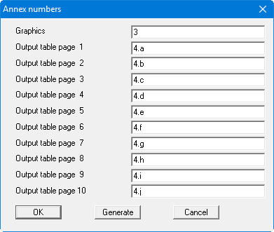
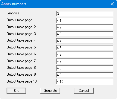
The number for the graphics is awarded by the program automatically if an annex number has already been entered in "Edit/General". The numbers for the output sheets can be easily generated by the program using the "Generate" button. You will then see a dialog box like this one:
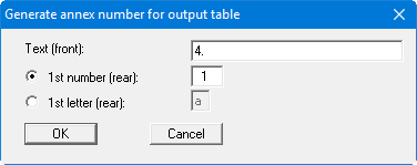
Enter the text to appear in front of the automatic numbering in the first input box; this can be a different number to the annex number for the graphics. It is then possible to select between numbering with numerals or a letter sequence. Activate the required command button and enter the first number or letter (in lower or upper case).
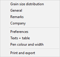
"Remarks" menu item
You can enter remarks to the tests in four lines. These lines will be entered at the bottom right of the form. In the dialog box you can enter the position of the text and the font size. The "Remarks" heading can be edited or deleted by going to the menu item "Output preferences/Texts + table" and pressing the "Silt and clay etc." button (see Section 6.4.2).
"Company" menu item
You can enter your company address in four lines. These lines will be entered at the top left of the form. Additionally, you can enter the position of the text and the font size.
"Undo" menu item
If you have carried out any changes to dialog boxes or moved objects to a different position on the screen after selecting the "Output preferences/Move objects" menu item or using the [F11] function key, this menu item will allow you to undo the movements. This function can also be reached by using the key combination [Alt] + [Backspace] or the appropriate tool in the toolbar (see Section 6.3.9).
"Restore" menu item
When this menu item is selected the last change made in a dialog box or the last change in the position of objects, which you undid using the menu item "Edit/Undo" will be restored. This function can also be reached by using the key combination [Ctrl] + [Backspace] or the appropriate tool in the toolbar (see Section 6.3.9).
"Preferences" menu item
You can activate or deactivate the undo functions.
Graphics preferences menu
"View output table"/"View diagram" menu items
The default screen visualisation is the grading curve graphics. If you go to the "View output table" menu item, the following dialog box opens:
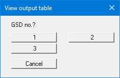
The "1", "2" etc. buttons represent the tests entered. A log page displaying the most important test data opens for each test. They can be printed via the menu item "File/Print and export" (see Section 6.1.9).
If you are viewing the output table, you can navigate between the output tables for the individual tests using the arrow tools in the toolbar. To return to the graphical visualisation of the grading curves, click on the now active menu item "View diagram" or simply on the tool. You can move between the output table and the graphical visualisation using this tool.


"Preferences" menu item
After selecting this menu item, a dialog box appears, in which you can edit preferences for
graphical presentation. All preferences made here can be saved at the program level using the "Graphics preferences/Save graphics preferences" menu item in a file named "GGU-SIEVE.alg". The preferences are then automatically loaded when the program is started.
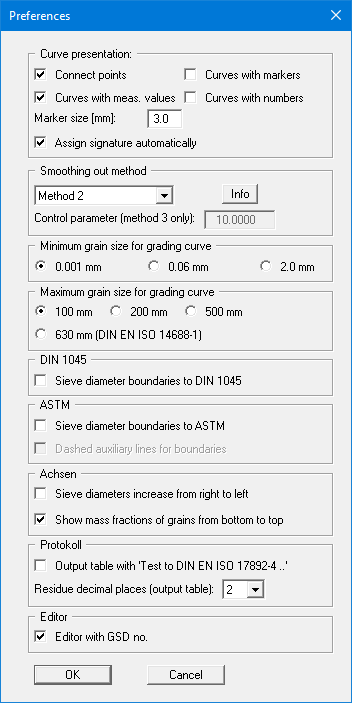
"Curve presentation" group box:
By activating the appropriate check boxes the measured data can be visualised as a grading curve, provided with markers at given intervals or directly attached to the measured data.
Each grading curve uses a different marker, thus ensuring simple differentiation between several grading curves, even on monochrome printouts. The marker size is user-defined. Instead of markers, the curves can also be labelled at their start and finish with the test numbers they represent.
If you want to define yourself which marker/signature should be used to display a grading curve, deactivate the "Assign signature automatically " check box. A selection menu then appears in the editor for each grain size distribution, which can be used to assign 10 different signatures.
"Smoothing out method" group box
You can choose between 4 methods, which are explained in the info box.
No smoothing = no smoothing
Method 1 = strict Bezier spline
Method 2 = "loose" Bezier spline
Method 3 = rational spline interpolation
Smoothing out methods 2 and 3 produce very round curves. The deviations between the measured values and the displayed grading curves become visible when the measured values of the test are marked.
For method 3, smoothing can be influenced by the "Control parameter". The value of the control parameter may only be in the range between > -1.0 and < 1000.
If you display the proportions T/U/S/G [%] in the diagram table, the proportions are determined from the curve. To obtain a more accurate approximation, change the Smoothing out method here or switch to "No smoothing".
"Minimum grain size for grading curve" group box
For coarse sample material, you can reduce the evaluation range for the fine grain component in the graphics in order to be able to select a better representation of the coarse grain range.
"Maximum grain size for grading curve" group box
For very coarse sample material you have the option of extending the evaluation range for the coarse grain component shown in the graphics. Additionally, it is possible to activate a display containing the grain component up to 630 mm diameter to EN ISO 14688-1 (= blocks).
"DIN 1045" group box
If you activate the "Sieve diameter boundaries to DIN 1045" check box, the [mm] specifications in the "Maximum grain size for grading curve" area above are adjusted according to the values from DIN 1045. You can then select the desired maximum grain size. The display of the grading curve in accordance with DIN 1045 always starts at 0 mm.
"ASTM" group box
After activating the "Sieve diameter boundaries to ASTM" check box the diameter boundaries can be displayed to suit the requirements of the American Society for Testing and Materials (ASTM). As a guidance aid you can also use dashed reference lines to mark the boundaries. If you have not used this previously, once you have activated the ASTM visualisation you will be asked whether the soil types and soil groups should also be determined compliant with ASTM. If you agree, the program automatically sets the corresponding check boxes, which you will find in the "Output preferences/Texts + table" menu item, to ASTM (see Section 6.4.2.3).
"Axes" group box
You can use the two check boxes "Diameter increase from right to left" and "Show mass proportions from bottom to top" to redesign the graphic according to your requirements
"Output table" group box
If the "Output table with 'Test to EN ISO 17892-4 ..'"check box is activated, the DIN EN ISO 17892-4 test type is displayed on the output table sheets.
You can specify the number of decimal places for the residue in the output table.
"Editor" group box
The buttons for the tests entered via "Edit/Grain size distribution" are labelled with the corresponding test number. If you deactivate the "Editor with GSD no." check box, the buttons are labelled with the entered designation. However, only the first 8 characters are used for this.

"Refresh and zoom" menu item
The program works on the principle of What you see is what you get. This means that the screen presentation represents, overall, what you will see on your printer. In the last consequence, this would mean that the screen presentation would have to be refreshed after every alteration you make. For reasons of efficiency and as this can take several seconds for complex screen contents, the screen is not refreshed after every alteration.
If, e.g., after using the zoom function (see below), only part of the image is visible, you can achieve a complete view using this menu item.
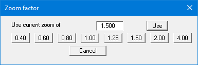
A zoom factor between 0.40 and 4.00 can be entered in the input box. By then clicking on "Use" to exit the box the current factor is accepted. By clicking on the "0.40", "0.60", etc. buttons, the selected factor is used directly, and the dialog box closed.
It is much simpler, however, to get a complete overview using [Esc]. Pressing [Esc] allows a complete screen presentation using the zoom factor specified in this menu item. The [F2] key allows screen refreshing without altering the coordinates and zoom factor.
"Zoom info" menu item
By clicking two diametrically opposed points you can enlarge a section of the screen in order to view details better. An information box provides information on activating the zoom function and on available options.
"Pen colour and width" menu item
For reasons of clarity, different colours are used as default for graphic presentation of the gradation curves, as well as the type of dashing. With this menu item you can alter the preferences to suit your wishes.
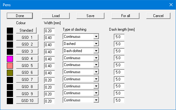
The pen width, line type and dashing can be edited for the grading curves and, after clicking the buttons with the GSD numbers, the pen colours be adapted. If the same line colour is to be used for all grading curves, press the "For all" button and specify the required colour. The pen preferences can be saved as an ".stf" file, or be loaded from such, using "Save" and "Load", to give a variety of pen combinations.
On monochrome printers (e.g. laser printers), colours are shown in a corresponding grey scale. Graphic elements employing very light colours may be difficult to see. In such cases it makes sense to edit the colour preferences.
"Legend font selection" menu item
With this menu item you can switch to a different true-type font. All available true-type fonts are displayed in the dialog box.
"Font size selection" menu item
You can edit font sizes of text within the various graphic elements.
"Mini-CAD toolbar" menu item
Using this menu item, you can add free text to the graphics and add lines, circles, polygons and images (e.g. files in formats BMP, JPG, PSP, TIF, etc.). PDF files can also be imported as images. A pop-up menu opens, the icons and functions used are described in more detail in the Mini-CAD manual saved in the 'C:\Program Files (x86)\GGU-Software\ Manuals' folder during installation.
"Toolbar preferences" menu item
After starting the program, a horizontal toolbar appears below the program menu bar. If you would rather work with a popup window with several columns, you can specify your preferences using this menu item. The smart icons can also be switched off.
At the bottom of the program window, you find a status bar with further information. You can also activate or switch off the status bar here. The preferences will be saved in the "GGU-SIEVE.alg" file (see menu item "Graphics preferences/Save graphics preferences") and will be active at the next time the program is started.
By clicking on the tools (smart icons) you can directly reach most of the program functions. The meaning of the smart icons appears as a text box if you hover with the mouse pointer over the tools. Some of the tool functions can be activated from the normal menu items.
"Zoom out"
If you have previously zoomed in, this tool returns to a full screen display.

"Zoom (-)"/"Zoom (+)"
With the zoom functions you can zoom in or out of parts of the image, by clicking the left mouse button.

"Undo"
If you have carried out any changes to dialog boxes or edited the position or size of an element on the output sheet ([F11] or used "Output preferences/Move objects"), you can undo the last changement with this tool.

"Restore"
If you have previously undone a changement, you can restore with this tool.

"Copy/print area"
Use this tool to copy only parts of the graphics in order to paste them, e.g. to a report. You will see information on this function and can then mark an area, which is copied to the clipboard or can be saved in a file. Alternatively you can send the marked area directly to your printer (see "Tips and tricks", Section 5.5).

"Diagram/output table"
By clicking on this icon you can switch between the tabular representation and the graphics representation.

"GSD output table up"/"GSD output table down"
Using this icon, you can navigate between the individual pages in the tabular representation.

"Load graphics preferences" menu item
You can reload a graphics preference file into the program, which was saved using the "Graphics preferences/Save graphics preferences" menu item. Only the corresponding data will be refreshed.
"Save graphics preferences" menu item
Some of the preferences you made with the menu items of the "Graphics preferences" menu as well as the inputs using the "Edit/Company" menu item can be saved to a file. If you select "GGU-SIEVE.alg" as file name and save the file on the same level as the program, the data will be automatically loaded the next time the program is started and need not be entered again.
If you do not go to "File/New" upon starting the program, but open a previously saved file instead, the preferences used at the time of saving are shown. If subsequent changes in the general preferences are to be used for existing files, these preferences must be imported using the menu item "Graphics preferences/Load graphics preferences".
Output preferences menu
"Page size" menu item
The default page set-up is A4 (landscape) when the program is started. You can edit the page format in the dialog box.
"Texts + table" menu item
Central preferences
After clicking on this menu item, the following dialog box appears:
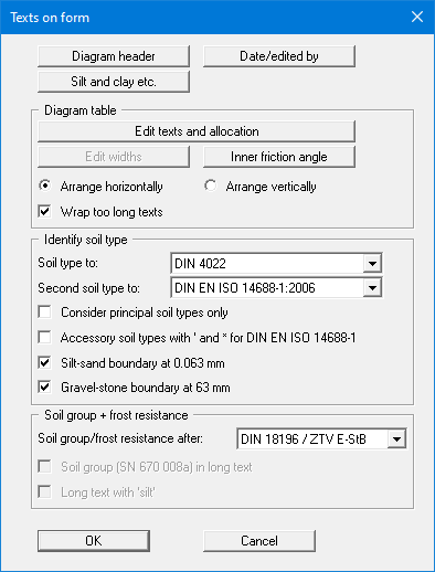
"Diagram header"
You can edit, or accept, the default wording, e.g. the heading, report no. and annex number. Further to this, you can rotate the alignment of the report number and the annex number.
"Date/edited by"
The default terms for "Date" and "Edited by" can be altered.
"Silt and clay etc."
If this button is pressed the headings of the grain size distribution diagram and the "Remarks" element can be altered.
The "Reset" buttons in the "Diagram header", "Date/edited by" and "Silt and clay etc." dialog boxes reset the labelling to the defaults. If you have retroactively changed the language, you will get the internal program translations.
"Diagram table" group box
In the "Diagram table" group box in the above "Texts + table" dialog box the required texts, text allocations and type of visualisation can be edited.
"Edit texts and allocation"
A dialog box opens for specifying the parameters and properties to be displayed in the diagram table. It is possible to display up to a maximum of 11 lines. The sequence corresponds to the numbering in the following dialog box.
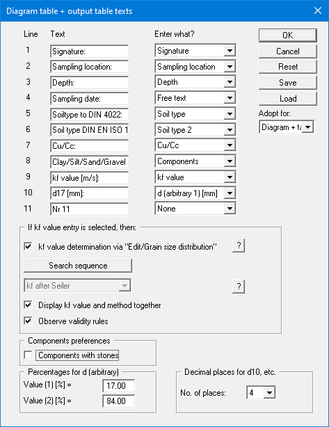
In the "Text" boxes a text must be entered by hand which is later used as a description. After clicking the arrows in the "Enter what?" column the values or text in the drop-down list entered or determined by the program can be allocated to the to the rows of the diagram table.
Lines with a "None" allocation are not displayed.
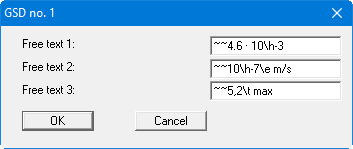
If information needs to be added to the table that is not found in the default texts in the table, a "Free text" can be used. In the menu item "Edit/Grain size distribution" you will then see an additional "Further input" button and can enter text according to your requirements in the dialog box.
In the Free texts you can make input with superscript or subscript numbers or letters using the conventions described below. To start the text, enter two '~~' characters. Superscripts and subscripts are activated using the backslash combinations '\h' and '\t'. If you need to use normal characters again following the superscripts or subscripts, follow them by '\e' before continuing normally (see file "Free texts with superscript-subscript.kvs").

The kf value is determined in accordance with the Merkblatt Anwendung von Kornfiltern an Bundeswasserstraßen (MAK) (Fact Sheet for the Application of Grain Filters on Waterways), published by the Bundesanstalt für Wasserbau (BAW) in Karlsruhe (2013).
If you want to display the kf value in the diagram table, you can select one of the various determination methods for all grain size distributions in the following group box. However, the check box "kf value determination via "Edit/ Grain size distribution"" is activated by default. You can then select different methods in the editor of the respective grain size distribution or, if "Automatic" is set there, have the system search for the appropriate method. You can change the search sequence by clicking on the corresponding button.
If you leave the "Display kf value and method together" check box activated, the method used is also displayed when a kf value entry is made in the diagram table. The respective validity rules should be observed, which is why the check box is activated by default.
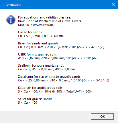
More detailed explanations of the methods can be found in an info box, which you can access by clicking on the "?" button:
If you are working in the stone area, you can expand the automatic display of the soil components in the diagram table accordingly by activating the "Components with stones" check box. You must adapt the table text "Clay/Silt/Sand/Gravel [%]:" manually.
Visualisation of the passages at d10, d30, d50 and d60 can be selected from the list. It is also possible to display the passages for any two percentage values. To do this, select the text allocation "d (arbitrary 1) [mm]" (see line 10 in the above dialog box) and enter the required percentage in the bottom group box. The text in the left column must be adjusted accordingly. The number of places after the decimal point can be selected for displaying the passages.
The "Reset" button resets the labelling and allocations of the results table to the defaults. If you have retroactively changed the language, you will get the internal program translations. Your texts and allocation can be saved in a "*.ktx" file using the "Save" button and opened again using the "Load" button. In addition, you can specify whether the current texts and properties allocations are applied to the diagram and/or the output table.
"Edit widths"
If the table is arranged vertically, a fixed width for each column can be defined using this button. Please note, however, that the total width of the table needs to fit into the layout of your output sheet. In order to achieve a uniform distribution within the specified total width, e.g. as defined using [F11], click the "All the same width" button.
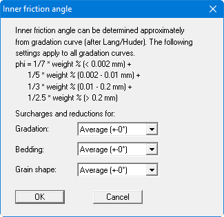
"Inner friction angle"
If the program is to estimate the inner friction angle, surcharges and reductions can be taken into consideration here:
"Arrange horizontally"/"Arrange vertically"
This command button defines the alignment of the diagram table.
"Wrap too long texts"
The program adapts the font size of the texts in the columns and rows automatically to the space available. The text may therefore appear very small for long input. If this check box is activated, the font size remains constant, but the text is wrapped and shown on several lines if necessary.
"Identify soil type" group box
Preferences for the evaluation and visualisation of the test results can be defined in this group box in the above "Texts + table" dialog box.
"Soil type to:"
The soil type can be determined to the DIN 4022 or the EN ISO 14688-1 in the 2006 or 2020 edition. In addition, the soil types can be determined using the SEP (Schichten Erfassungs Programm) system of the Niedersächsisches Landesamt für Bodenforschung (Geological Survey of the State of Lower Saxony) or to ASTM (American Society for Testing and Materials).
"Second soil type to:"
You can visualise two soil types in the diagram table, for example to old and new DIN. Choose the standard for determining the second soil type here.
Both input boxes are available in the editor box for each grain size distribution. However, the soil types are only shown in the diagram table if "Soil type" and "Soil type 2" have been allocated a table row in the "Edit texts and allocations" dialog box.
"Consider principal soil types only"
Normally, when determining the soil type, the program also gives the subdivisions for the sand and gravel ranges as fine/medium/coarse sand or fine/medium/coarse gravel. Activate this check box to suppress this function. Sand or gravel components are then summarised as one fraction in the soil type.
If you have made any changes here the "Determine soil type" button must be pressed again in the respective test number for existing grain size distributions.
"Accessory soil types with ' and * for EN ISO 14688-1"
If the soil types are determined to the EN ISO 14688-1 the accessory soil types can be further differentiated into slightly ( ' ) and heavily ( * ) by activating this check box. This is not provided for in the new standard but adds clarity.
"Silt-sand boundary at 0.063 mm"
The program determines the silt component at the silt-sand transition, which is 0.060 mm in the diagram according to DIN. If the final value is entered for the 0.063 mm sieve for a pure sieving, the transition to silt would not be reached and the program would not take the silt component into consideration when determining the soil type. By activating this check box, the silt content is determined at 0.063 mm. The graphic is adjusted accordingly.
"Gravel-stone boundary at 63 mm"
The program determines the stone component at the gravel-stone transition, which is 60 mm in the diagram according to DIN. The boundary transition is moved to 63 mm by activating this check box.
"Soil group + frost resistance" group box
Further preferences for the evaluation and visualisation of the test results can be defined in this group box in the above "Texts + table" dialog box.
"Soil group/frost resistance after:"
Here, it is possible to choose between DIN 18196/ZTV E-StB, SN 670 008a (Swiss Norm) or USC (Unified Soil Classification) as the method of determination.
"Soil group (SN 670 008a) in long text"
If you are using the Swiss standard a long text version of the soil group can be specified here.
"Long text with 'silt'"
If the soil group is displayed as a long text according to the Swiss standard the usual Swiss term "silt" can be used instead of the German "Schluff".
"Margins" menu item
In the default program preferences, the output sheet is shown with cutting borders. For output to an A4 printer, a reduction of the printer output is generally necessary, as proprietary printers cannot fully cover an A4 page. The margin preferences can be defined in the following dialog box.
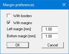
By deactivating the "With borders" check box and with an appropriate choice of left and lower margins, it is generally possible to create a non-reduced printer output. It may be necessary to also adapt the page height and/or width on some printers (see Section 6.4.1).
If you also deactivate the "With margins" check box, the thicker border around all the graphic elements on the output sheet will be removed. You can create a completely new arrangement on the form by moving the individual graphic elements.
"Position info" menu item
The positions and layout of the individual elements on the output sheet can be altered using the following menu items. This menu item provides information on the options for altering the position and layout more quickly using the mouse.
"Title (change position)" menu item
This menu item is invisible if you are in the output table view. The position and layout of the title element can be altered via the dialog box for this menu item, if the "Title display" check box is activated.
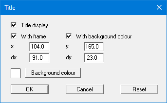
The position of the element on the output sheet and its size can be defined or edited by means of the variable's "x" and "y", "dx" and "dy". The element can be provided with a frame and a background colour to suit your personal requirements. If the element needs to be returned to its original condition, this can be done using the "Reset" button. Alternatively, you can alter the size and shape of the element using the mouse (see menu item "Output preferences/Move objects", Section 6.4.18).
The heading shown in the title element can be edited in the menu item "Output preferences/Texts + table", "Diagram header" button (see Section 6.4.2). The texts "Project (1st line)" and "Project (2nd line)" are entered immediately after double-clicking the element or using the menu item "Edit/General" (see Section 6.2.10).
"Grading curve" menu item
A dialog box opens that is almost identical to that for the previous menu item. The same preferences can be specified in this box as in that described in Section 6.4.5. Because the grading curve is the central graphical element, it cannot be switched off. Proceed as described above to alter the position or layout of the "Grading curve" element.
"Company" menu item
Almost the same dialog box opens with the same preference options as that described in the "Output preferences/Title (change position)" menu item (see Section 6.4.5). Simply proceed as described there to edit the "Company" element.
The input for this element can be edited immediately after double-clicking on the element or via the menu item "Edit/Company" (see Section 6.2.13).
"Examination no. etc." menu item
Almost the same dialog box opens with the same preference options as that described in the "Output preferences/Title (change position)" menu item (see Section 6.4.5). To edit the "Examination no. etc.", element, simply proceed as described there.
The input for this element can be edited immediately after double-clicking on the element or via the menu item "Edit/General" (see Section 6.2.10). For this element you also have the option of adapting the texts in front of the input boxes to suit your needs. Go to the menu item "Output preferences/Texts + table", "Diagram header" button (see Section 6.4.2.1).
"Annex and report" menu item
Almost the same dialog box opens with the same preference options as that described in the "Output preferences/Title (change position)" menu item (see Section 6.4.5). To edit the "Annex and report" element, simply proceed as described there.
The input for this element can be edited directly by double-clicking the element or by going to the menu item "Edit/General" (see Section 6.2.10). Here, you can also alter the texts in front of the input boxes to suit your needs. This is also possible by going to the menu item "Output preferences/Texts + table", "Diagram header" button (see Section 6.4.2.1). Using the latter item it is also possible to rotate the texts by 90°, but can also be achieved by opening the element directly by double-clicking.
"Diagram table" menu item
This menu item is invisible if you are in the output table view. Almost the same dialog box opens with the same preference options as that described in the "Output preferences/Title (change position)" menu item (see Section 6.4.5). To edit the "Diagram table" element, simply proceed as described there.
"Remarks" menu item
This menu item is invisible if you are in the output table view. Almost the same dialog box opens with the same preference options as that described in the "Output preferences/Title (change position)" menu item (see Section 6.4.5). To edit the "Remarks" element, simply proceed as described there.
The input for this element can be edited immediately after double-clicking on the element or via the menu item "Edit/Remarks" (see Section 6.2.12). The "Remarks" heading can be edited or deleted by going to the menu item "Output preferences/Texts + table" and pressing the "Silt and clay etc." button (see Section 6.4.2).
"Edited by + date" menu item
This menu item is invisible if you are in the output table view. Almost the same dialog box opens with the same preference options as that described in the "Output preferences/Title (change position)" menu item (see Section 6.4.5). To edit the "Edited by + date" element, simply proceed as described there.
The input for this element can be edited immediately after double-clicking on the element or via the menu item "Edit/General" (see Section 6.2.10). For this element you also have the option of adapting the texts in front of the input boxes to suit your needs. Go to the menu item "Output preferences/Texts + table", "Date/edited by" button (see Section 6.4.2.1).
"Output table (results)" menu item
This menu item is invisible if you are in the grading curve graphics view. Almost the same dialog box opens with the same preference options as that described in the "Output preferences/Title (change position)" menu item (see Section 6.4.5). To edit the "Output table (results)" element, simply proceed as described there.
"Output table (sieve analysis)" menu item
This menu item is invisible if you are in the grading curve graphics view. Almost the same dialog box opens with the same preference options as that described in the "Output preferences/Title (change position)" menu item (see Section 6.4.5). To edit the "Output table (sieve analysis)" element, simply proceed as described there.
"Output table (hydrometer analysis)" menu item
This menu item is invisible if you are in the grading curve graphics view. Almost the same dialog box opens with the same preference options as that described in the "Output preferences/Title (change position)" menu item (see Section 6.4.5). To edit the "Output table (hydrometer analysis)" element, simply proceed as described there.
"General" menu item
Almost the same dialog box opens with the same preference options as that described in the "Output preferences/Title (change position)" menu item (see Section 6.4.5). To edit the "General" element, simply proceed as described there.
In the program default setting this element is deactivated. If the "General display" check box is activated in the dialog box for this menu item, the element is displayed in the graphical visualisation of the grading curves on the output sheet. The text can be edited by double-clicking within the element. An editor box opens in which a heading can be entered and the type of presentation of the file name be selected.
"Reset all" menu item
With this button, all preferences for the aforementioned elements which may have been edited with the previous menu items, will be reset to the program defaults.
"Move objects" menu item
When you go to this item you can move the various objects with the aid of the mouse. Move the mouse over the object to be moved. When you are located above a moveable object the mouse pointer appears in the shape of a cross. You can now press and hold the left mouse button and drag the object to the required position.
After going to this menu item only one object at a time can be moved using the mouse or its size be altered.
In order to move or edit several objects, this function can be more quickly activated by pressing [F11] or the icon.

The size of an object can also be altered using this menu item or the [F11] key. If you move over the frame of a changeable object after activating this function the mouse assumed the shape of a double-headed arrow. Hold the left mouse button and move the frame until the object has reached the required size. To retain the ratio of the sides, pull at one corner only. If on one side only is pulled the object will become higher or wider.
The last change made in the position or size of an object can be undone using [Back] or by clicking the icon.

Special menu
General notes
A maximum of 10 tests can be edited and presented using the "Edit/Grain size distribution" menu item. A limit of ten tests is necessary, as more than this will not fit in the diagram table on the form, together with the remarks to the tests.
An input of further 100 tests is possible using the "Special" menu. For these tests (to be called extra grain size distributions or extra GSDs), no entry in the diagram table is made. Only a legend will be shown, making possible an allocation of line type and test designation.
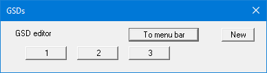
"Enter extra GSDs" menu item
Using this menu item you can enter extra GSDs. Input is almost completely the same as described in the "Edit/Grain size distribution" menu item (see Section 6.2.2) and need not therefore be further explained here. A total of 100 extra GSDs can be entered.
If you would like to enter boundary curves, it is much simpler to enter certain diameters as percentage values. For this purpose, the button

is available for sieving data input. If you click this button with the mouse, the text on the button will change to
.

All numerical input following the sieve diameters then corresponds to the sum of the passage in percent (also see Section 6.2.2.2, page 22, menu item "Edit/Grains size distribution", Sieve analysis input).
"Load extra GSDs" menu item
Extra grain size distributions previously saved using the menu item "Special /Save extra GSDs" can be opened separate from the primary record. If extra GSDs (".xkv") are already open they can be replaced by a new one by pressing the "New" button or appended to the existing grain size distribution using "Add".
"Save extra GSDs" menu item
Extra GSDs can be saved separate from the primary grain size distribution to have them available for other primary records. In this way it is possible to create several templates, for example for certain boundary ranges, which can be used as a background for examining grain size distributions (see the example file "boundary_01-e.xkv").
"Delete extra GSDs" menu item
After a confirmation prompt, you can delete all extra GSDs.
"Extra GSDs preferences (1)" menu item
With this menu item you can define important preferences for extra GSDs. You will see the following dialog box:

In the "Curve representation" group box you can specify the smoothing out procedure with which the GSDs are to be presented. A further explanation can be found in the menu item "Graphics preferences/Preferences" in Section 6.3.2.
For the display of the extra GSDs, you can decide whether the grain distribution curve should be displayed as a line and/or with markers on the measured values.
You can use the "Extra GSDs pens" button at the bottom of the dialog box to set different pen colours, widths and, if required, dashing for the display of the first 5 extra grain size distributions (see figure below).
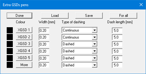
Use the "More" button to specify a common display type for all subsequent extra grain size distributions (6 - 100). Use the "For all" button to select a common colour for all 100 extra grain size distributions in one step.
It is often desirable when visualising boundary curves to hatch areas. The hatching is defined in the "Hatch what" in the dialog box shown above. Here you can define 3 areas to be hatched, by selecting the desired GSD for the hatch boundary from the input boxes:
Hatch between the lower diagram edge and an extra GSD.
Hatch between the upper diagram edge and an extra GSD.
Hatch between two extra GSDs.
Upon selecting "None", no hatching will be entered for this area. With the "Hatch lines" button varying hatch lines can be created.
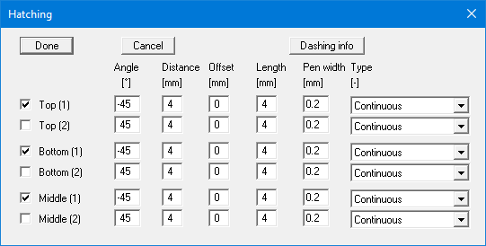
Hatching can consist of two lines, e.g. in order to create a cross-hatch. The curves for the required ranges are activated using the check boxes. Further information is available by pressing the "Dashing info".
Alternatively, it is possible to fill the areas with a certain colour. The colour is defined in the "Hatch colours" group box of the Extra GSD box. Click on the corresponding buttons and select the required colour from the colour dialog box. The current colour is shown in the small box beside the buttons.
The preferences described above for line and/or colour hatching are only active if the requisite check box is activated in the "Hatch how?" group box.
"Extra GSDs preferences (2)" menu item
This menu item is available if you would like to emphasise a 2nd area between 2 grain lines differently. You will see the following dialog box:
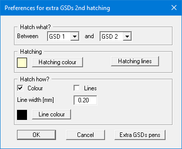
You can set a desired colour and hatching line for this 2nd hatching area. You can also assign a different colour, pen width or hatching line to the selected boundary hatching lines using the "Extra-KVS pens" button (see Section 6.5.6, page 56).
"Extra GSDs output table" menu item
In complete analogy to the "File/Print 'simple' output table" menu item (see Section 6.1.6), an extra GSDs output table can be printed.
"Load GSDs as extra GSDs" menu item
Grain size distributions already entered as normal grain size distributions and saved as ".kvs" files can be imported as extra grain size distributions using this menu item. This allows you to collate all grading curves to a grading band.
First decide whether the grading curves are to be opened as new extra grain size distributions or appended to the existing extra grain size distributions. Then select the required file in the file selector box. It is also possible to mark and open several files at once. You will see a message on the number of files imported and the grading curves they contain.
"Extra GSDs legend" menu item
If extra grain size distributions have been entered, a legend containing all extra GSDs can be displayed. If the "Show extra GSDs legend" check box is activated, you can edit the position and representation in the dialog box for this menu item.

You can define and edit the position of the legend using the values "x" and "y". The size of the legend is controlled using "Font size" and "Max. no. of rows"; where necessary, several columns are used. The fastest way to modify the position of the legend is to press the [F11] function key and then to drag and drop the legend to the new position holding the left mouse button.
The names and defined line types (colour, dotted, etc.) of the extra grain size distributions are displayed below the heading in the legend. The preferences for the pens can be edited in the above dialog box using the "Edit extra GSDs pens" button, analogous to the menu item "Special/Extra GSD s preferences", "Extra GSDs pens" button (see Section 6.5.6, page 56).
"Inner friction angle legend" menu item
Using this menu item you can define a legend for the surcharges and reductions for the inner friction angle, if you have activated the "Show legend" check box. The legend can only be displayed if automatic estimation of the friction angle is activated in "Edit texts and allocations", one row below "Enter what?" in the menu item "Output preferences/Texts + table".
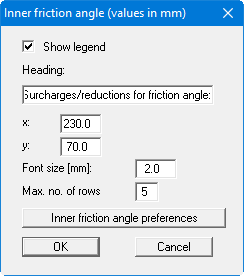
You can define and edit the position of the legend using the values "x" and "y". You control the size of the legend using "Font size" and "Max. no. of rows"; where necessary, several columns are used. The fastest way to modify the position of the legend is to press the [F11] function key and then to pull the legend to the new position with the left mouse button pressed.
After going to this menu item it is possible to edit the surcharges using the "Inner friction angle preferences" button (see menu item "Output preferences/Texts + table", "Inner friction angle" button, Section 6.4.2.2, page 48).
"Check grading curve range" menu item
You can define a grading curve range with 2 extra grain size distributions. Using this menu item, you can determine and display any deviation from the defined range for all existing grading curves and extra grading curves.
Info menu
"Copyright" menu item
You will see a copyright message and information on the program version number.
The "System" button shows information on your computer configuration and the folders used by GGU-SIEVE.
"GGU on the web" menu item
Using this menu item, you can access the GGU Software website: www.ggu-software.com.
Get information on updates and modifications on a regular basis from your program module page. On the "Changelogs" subpage, you can also subscribe to an e-mail notification that informs you of all changes monthly.
"GGU support" menu item
This menu takes you directly to the GGU-Software Support Portal.
"Maxima" menu item
You will see information on the default program maxima.
"Help" menu item
The GGU-SIEVE manual is opened as a PDF document. The help function can also be accessed using the [F1] function key.
"What's new?" menu item
You will see information on program improvements in comparison to older versions.
"Language preferences" menu item
This menu item allows you to switch the menus and the graphics from German to English and vice versa. To work in German, deactivate the two check boxes "Dialoge + Menüs übersetzen (translate dialogues, menus)" und "Graphiktexte übersetzen (translate graphics)".
Alternatively, you can work bilingually, e.g. with German dialog boxes but with graphic output in English. The program always starts with the language setting applicable when it was last ended.
Index
A
Accessory soil types,
define representation preferences 49
overline for old DIN 18
Alignment, diagram table 48
American Society for Testing and Materials 48
Annex number,
edit element 52
enter 35
generate for output table sheets 36
rotate by 90° 44, 52
ASTM,
define graphics visualisation 39
select for soil type determination 48
B
Blocks, consider in soil type determination 39
Borders, turn on/off 50
Boundary curves, define 55
C
Calculation operations,
in input boxes with numbers 8
Clipboard 14
Coefficient of plasticity, enter 18
Colours,
define for extra GSDs pens 59
define for grading curve pens 41
Column width, diagram table 48
Company,
edit element 51
enter address 37
Context menu, open 7
Control parameter, smoothing GSDs 39
Copy/print area 10, 14, 42
Cu/Cc, activate display in diagram table 45
Cumulative weight, activate 16
D
Dashing, grain range 57
Decimal places,
specify for passages 47
specify for residues in output table 39
Delete,
all extra GSDs 56
all GSDs 30
individual GSDs 19
Diagram header,
change texts of input boxes 44
edit element 51
enter 35
Diagram table,
alignment 48
define entries 45
define text length 48
edit element 52
edit text allocation 45
load/save text allocation 48
DIN 1045,
define evaluation range 39
DXF file,
export 14
import via Mini-CAD 5
E
Editor window, output table 12
EMF format 14
EN ISO 14688-1,
activate block display 39
activate for soil type determination 48
Evaluation range of GSD,
activate to ASTM 39
activate to DIN 1045 39
Evaluation range of GSD, reduce/extend 39
Examination number,
edit element 52
enter 35
fade out 44
Extra GSDs,
combine existing GSDs 58
delete all 56
display as boundary curves 57
display as grain range 58
enter 55
pen preferences 59
preferences 56
save/load 55
F
File,
combine several to one 58
display name in legend 53
extension explanation 9
load/save 11
Filter rules, display Terzaghi/USBR 19
Filter stability verification,
after Cistin/Ziems 33
of geotextile filters 34
Font selection 41
Font size, define for graphic elements 41
Free text,
define input box for diagram table 46
define superscripts or subscripts 46
enter 18
Frost resistance,
activate display in diagram table 45
select determination method 49
Function keys 9
G
GGU-CAD file, export 14
GGU-FILTER-STABILITY,
export possibilities 32, 33, 34
GGUMiniCAD file, export 14
Grading curve range, check 60
Grading curves,
edit values graphically 30
pen preferences 41
smoothing out methods 39
Grain diameters,
display in a message box for all passages 19
Grain filters, application on waterways 31, 33, 47
Grain index, activate display in diagram table 45
Graphics, add via Mini-CAD 42
Gravel-stone boundary, define 49
GSD diagram,
activate representation 37
edit element 51
edit grain labelling etc. 44
GSDs (= Grain size distributions),
combine from several files 58
delete all 30
delete individual 19
enter/edit 16
load together 11
mix 30
specify sequence 16
swap sequence 29
H
Hatching, define for extra GSDs 57
Hydrometer,
enter reading 27
load/save reading intervals 27
save/load individual values 26
switch all GSDs to another Standard hydrometer 30
switch to another Standard hydrometer 26
I
Individual test,
delete 19
duplicate 19
load/save 19
output as ASCII file 19
output as table 19
save as ASCII file 19
Inner friction angle,
activate determination 45
activate display in diagram table 45
define surcharges/reductions 48
display surcharges/reductions in legend 60
IP, enter 18
K
kf value,
activate display in diagram table 45
display in a message box for all methods 19
select determination method for all 47
select method for each GSD separately 19
switch validity rules on/off 47
L
Language preferences 6, 61
Layout, define for output sheet 43
Legend,
activate for extra GSDs 59
activate for inner friction angle 60
alter position/size using mouse 54
Licence protection 5
Liquid limit, enter 18
M
Manual, open as PDF file 61
Marker-signature,
change preferences 39
deactivate automatic assignment 39
Maximum grain size for curves,
evaluation range to DIN 1045 39
extend evaluation range 39
Measured data, display 39
Metafile, export 14
Mini-CAD,
application explanations 42
export file 14
Minimum grain size for curves,
reduce evaluation range 39
Mouse click functions 7
N
Navigation, output table 43
O
Objects, alter position/size using mouse 54
Output preferences 12, 13
Output sheet,
alter position/size of individual elements
using mouse 50, 54
reset all elements to defaults 53
reset individual elements to defaults 51
Output table,
activate representation 37
automatic entry of test type 39
marking partial sum weighing 24
print for all GSDs 12
print for an individual GSD 37
print for extra GSDs 58
Overline for accessory soil types 18
P
Page,
copy/print section 10, 42
define format 43
define margins 50
Pagination, automatic 12
Pan weight, calculate 21
Partial mass sieving, enter 23
Partial sieving,
activate to DIN EN 933-1 16
Passages,
activate display in diagram table 45
select percentages for display 47
PDF file, import via Mini-CAD 5, 42
Pen preferences,
for extra GSDs 59
for grading curves 41
Print,
graphics 13
output table 12
section 10, 14, 42
several files 15
Program,
load/save preferences 43
show default maximum values 61
show improvements 61
show information 61
R
Remarks,
edit element 52
edit labelling 44
enter 36
Report number,
edit element 52
enter for GSD diagram 35
rotate by 90° 44, 52
S
Scroll the screen 7
SEP Schichten Erfassungs Programm 48
Sieve analysis,
activate input boxes 20
activate partial mass sieving 23
enter/edit test data 21
Sieve data,
as residue in [g] 22
as sum of passage in [%] 22, 55
enter as cumulative weight 16
Sieves, save/load combination 22
Silt-sand boundary, define 49
Simple output table,
print for all GSDs 12
print for an individual GSD 19
Smart icons, for menu items 42
Smoothing out methods, grading curves 39
Soil components,
activate display in diagram table with stones 47
Soil groups to DIN 18196,
define Ip/wL 18
visualise as fill 19
Soil groups,
activate display in diagram table 45
select determination method 49
Soil properties, determine for export to
GGU-FILTER-STABILITY 32, 33, 34
Soil type,
activate display in diagram table 45
determined by the program 18
enter the same for all GSDs 29
select determination method 48
Special values, determine/display 19
Status bar main program, activate 42
Stones,
activate component display in diagram table 47
Subscripts, use in diagram table 46
Suffosion safety verification,
after Kenney/Lau and Burenkova 32
by separating a GSD 31
Superscripts, use in diagram table 46
Swiss standard SN 670 008a 49
System, show information 61
T
Terzaghi, display filter rules 19
Test numbers,
activate labelling with 39
sequence 16
Test results, save in file 12
Texts in diagram table,
define length/size 48
enter/edit 45
Toolbar, edit for menu items 42
Translation,
activate 61
display retroactively for output sheet 44
display retroactively in result table 48
True-type font 41
U
Uniformity coefficient Cu,
display in a message box 19
USBR, display filter rules 19
USC Unified Soil Classification,
select for soil group determination 49
V
Version number, show 61
Versuchsergebnisse, als XML file, save 13
W
Wet analysis,
activate input boxes 25, 27
enter/edit test data 27
What you see is what you get 40
wL, enter 18
Z
Zoom factor, define for full-screen display 40
Zoom function, activate 40, 42