
Using this menu item, you can edit cone penetration tests. A dialog box opens allowing a new cone penetration test to be entered by pressing the "New" button, or an existing cone penetration test to be selected for editing by clicking the button for the respective test. For example, if you open the "Ex_CPT 2.bop" example file the following dialog box opens after clicking "CPT 1":
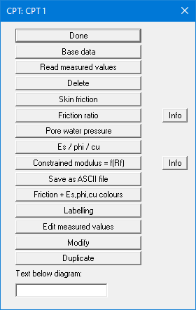
Several diagrams can be created for a cone penetration test evaluation. The cone resistance diagram is the central element of the cone penetration test and is always visualised. Visualisation of the skin friction, friction ratio, pore water pressure, constrained modulus, friction angle and undrained shear strength can be switched on or off. The cone penetration test editor box shown above can also be opened directly by double-clicking in the cone resistance diagram on the screen. When performing actions via the "Edit" menu or simply moving objects using [F11], click in the cone resistance diagram as the central element of the cone penetration test. The following actions can be performed using the buttons and input boxes in the dialog box:
-
"Done"
You will arrive back at the previous dialog box. Alterations will be accepted. -
"Base data"
You can enter or edit the base data for the corresponding CPT.
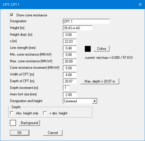
With "Height" and "x" you enter the position of the cone penetration test (CPT). Here, you can also enter a "Height displacement" (see "Input/Stratigraphic log", "Base data" dialog box). "Line strength" designated the width with which the curve is drawn. With the "Colour" button you can alter the pen colour.
"Min. cone resistance", "Max. cone resistance" and "Cone resistance increment" control the cone resistance axes. "Width of CPT" and "Depth of CPT" control the depth and width of the cone resistance diagram on the page. The maximum depth achieved is shown on the right-hand button after the measured values are imported. Click the button to transfer the value to the "Depth of CPT" box. The vertical subdivision of the diagram is defined by the "Depth increment"; here, it is subdivided after each metre. Furthermore, you can change the font size of the axes.
Alignment of the designation and height of the selected cone penetration test can be edited using the drop-down menu. At the bottom of the dialog box, you can specify whether the absolute height should be additionally displayed or only the absolute height when displaying the depth data.
-
"Read measured values"
You can import the result data of a CPT from an ASCII file. The data in this file, which you will generally receive from the performing company, must contain one value per row (depth, cone resistance and, optionally, skin friction). After selecting a file with measured values, the following dialog box appears:
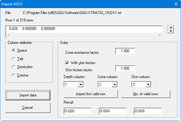
The current row of the ASCII file is shown at the top of the window. Using the arrows at the right you can move through the file. If the file also contains skin friction values, activate the "With skin friction" check box. When all input is correct, the result for this row will appear in the box below the columns. Otherwise "Error" will appear. You may then have to alter the column delimiter. If the file contains invalid as well as valid rows, these will be simply skipped when reading.
The program expects the values in MN/m². If the measured values are not in the correct dimension, you can enter a correction factor under "Cone resistance factor" and/or "Skin friction factor". Finally, select the "Import data" button. You will then see information on the number of rows read. You can then edit the CPT further or evaluate it.
-
"Delete"
After a security request the currently displayed test will be deleted. -
"Skin friction"
You can activate the skin friction display and set preferences for the skin friction values diagram. To do this, the following dialog box opens:
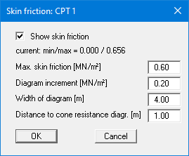
With "Distance to cone resistance diagr." you can control the distance of the skin friction diagram to the cone resistance diagram. Using the program defaults it will be displayed with a spacing of one metre (= 1 cm at a scale in x-direction of 1:100) to the left of the cone resistance diagram.
-
"Friction ratio"
The friction ratio can be calculated from the cone resistance and skin friction and displayed in a diagram. Clicking this button opens a dialog box analogous to the skin friction box. A list of the allocations of friction ratio values to certain soil types can be viewed by clicking on the neighbouring "Info" button. -
"Pore water pressure"
You can activate a pore water pressure representation and design the diagram according to your wishes. The following dialog box opens for this purpose:
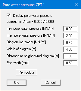
With "Distance to neighboured diagram" you control the distance of the pore water pressure diagram to the neighbouring diagram. The default setting of the program shows it at a one metre distance (= 1 cm at a scale of 1:100 in x-direction) to the right of the friction ratio diagram.
-
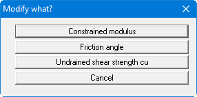
"Es / phi/ cu"
Three additional diagram types can be activated by pressing this button. The option box opens first:
"Contrained modulus":
To visualise the constrained modulus diagram, activate the "Show constrained modulus" check box. Two options are available for determining the constrained modulus:
1) To obtain the constrained modulus, the cone resistance qc is multiplied by a factor alpha depending on the friction ratio Rf. The factors are defined using the "Constrained modulus = f(Rf)" button described further below, which you can reach via the initial editor box.
2) Depending on the soil type determined via the soil identification diagram, the constrained modulus is derived from the factor alpha stored for the respective soil type and the cone resistance qc.
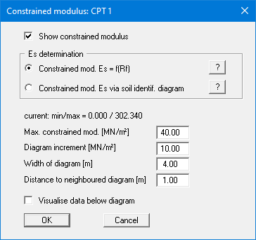
The lower part of the dialog box corresponds to that for skin friction. By activating the "Visualise data below diagram" check box, a legend containing the factors corresponding to the selected constrained modulus is displayed below the constrained modulus diagram.
"Friction angle":
In addition, you can have the friction angle displayed. Different equations are available to determine phi.
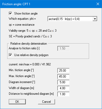
The boundary between cohesive and non-cohesive soils is defined via the soil identification diagram. You can specify whether the relative density of non-cohesive soils is to be determined up to the boundary line at the friction ratio value you set or via the relative density polygon defined in the "CPTs (soil index)" legend. You can also adjust the polygon there according to your needs.
The lower part of the dialog box corresponds to that for skin friction.
"Undrained shear strength cu":
You can show the undrained shear strength cu in an additional diagram. To achieve this, modify the visualisation to suit your wishes in the following dialog box. By pressing the "?" button, you are shown the equation used to determine the undrained shear strength.
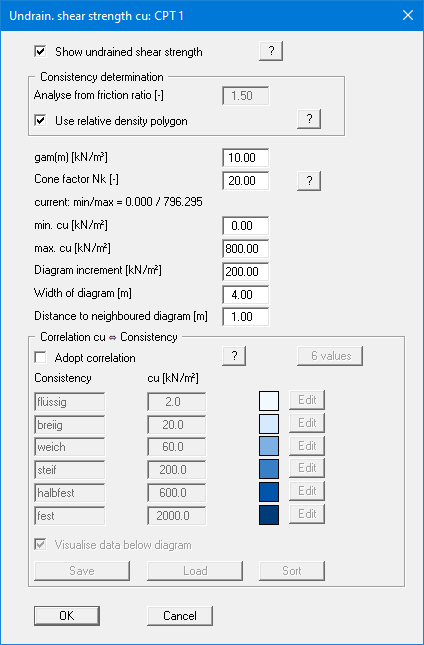
The boundary between cohesive and non-cohesive soils is defined via the soil identification diagram. You can specify whether the consistency of cohesive soils is to be determined from the boundary line at the value you have specified for the friction ratio or from the relative density polygon defined in the "CPTs (soil index)" legend. You can also adjust the polygon there according to your needs.
Alternatively, consistency can be defined using the correlation to cu, which can be activatedin the lower group box of the dialog box.
-
"Contrained modulus = f(Rf)"
Depending on the friction ratio Rf, the cone resistance must be multiplied by a factor to obtain the constrained modulus.
In the following dialog box, enter the friction ratio Rf up to which up to which the respective factor is to apply. The dialog box allows display of up to 8 value pairs. If more values are available, you can scroll through the table using "Forw." and "Back". If you want to change the number of value pairs, select the "Edit no. of values" button. If you want to insert a value pair, increase the number of value pairs and enter the value pair at the end of the table. Then select the "Sort" button. The table will be sorted by ascending Rf values. The sort function is always called after leaving the dialog box.
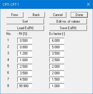
If you want to save the table, select the "Save Es(Rf)" button. If you then keep the default file name, "GGU-STRATIG.rfe", the values in the table will be automatically active at the next program start. If you would like to load values from a previously saved file, select the "Load Es(Rf)" button. A list of constrained moduli for certain soil types can be viewed by clicking on the neighbouring "Info" button.
-
"Save as ASCII file"
You can save the values (depth, cone resistance and optionally skin friction) as an ASCII file. -
"Friction + Es,phi,cu colours"
The area between the measured value curve and the vertical axis can be coloured. The settings are modified in this dialog box.
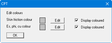
With reference to the colour presentation of cone resistance and friction ratio, please see the menu item "Input/Legends" ("CPTs (cone resistance)" legend, "CPTs (friction ratio)" legend and "CPTs (soil index)" legend).
-
"Labelling"
The individual diagrams (cone resistance, skin friction, friction ratio, constrained modulus, friction angle, undrained shear strength, pore water pressure) are labelled at the top. In this box you can change the default labelling -
"Edit measured values"
You can edit loaded values or enter values completely by hand. Use of the dialog box corresponds almost exactly to that of the "Constrained modulus = f(Rf)" dialog box described above. A "Sort" button is not present, the values will nevertheless be sorted automatically for increasing depth upon leaving the dialog box. In principle, the "Edit values" function can also be abused for other purposes. It is imaginable, e.g., to enter a water
content profile, which can also be colour-coded (see "CPTs (cone resistance)" legend).
It is also possible to create a bar chart with variable bar width etc. The only limit is your imagination. -
"Modify"
This button opens a dialog box which allows the measured value to be modified using a variety of operations involving constants. -
"Duplicate"
By clicking this button, you can duplicate the current cone penetration test. You will then find yourself in the "Base data" dialog box of the duplicated test. -
"Text below diagram"
In this field you can enter a text to be displayed below the cone penetration diagram. In order to create a line break, you must enter a "#" (e.g. No further progress#concrete).