
"Info" menu item
You will see information on the current system in a message box.
"Special preferences" menu item
The program performs a multitude of plausibility checks. After starting the analysis, the preferences specified by the user are displayed in an info box; for problematical preferences separate information or warning are displayed. It is therefore recommended to leave the "Show warnings in future" check box activated.
If you do not want to see the automatic display when the analysis starts, deactivate the check box. You can subsequently view your special preferences using this menu item.
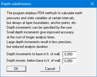
"Depth subdivisions" menu item
GGU-GABION uses the finite element method, which requires the system to be divided into a number of finite elements (rods) (see section 7.14). You can specify the size of these depth increments for the region above and below the base in front of wall.
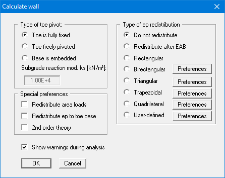
"Analyse" menu item
Start dialog box
Once you have entered all data required to fully describe the system it can be analysed. After going to the "System/Analyse" menu item a start dialog box, divided into three group boxes, opens (see below for descriptions). You can also initiate the analysis using the [F5] function key and see the same start dialog box.
When all preferences have been specified to your satisfaction press the "OK" button to start the analysis. The program first performs comprehensive plausibility checks on your input and notifies you of any inconsistencies. The actual analysis of the system then follows.
Once analysis is complete, the results are presented in message boxes and then visualised graphically on the screen.
"Type of toe pivot" group box
In the first group box of the start dialog box of the "System/Analyse" menu item you can specify the toe pivot. This is, of course, not possible in systems without geogrids. In such cases, the toe is always fully fixed.
In systems with geogrids, a subgrade modulus for the base can be entered in place of "Toe is fully fixed" or "Toe freely pivoted". Activate the "Base is embedded" check box and enter a subgrade reaction.
"Special preferences" group box
In the "Special preferences" group box of the start dialog box of the "System/Analyse" menu item you can specify whether any area loads should be included in an earth pressure redistribution. You may "Redistribute ep to toe base" and not, as is usual, to the load transition point.
For an analysis employing the global safety factors used in DIN 1054 (old), the load transition point can be calculated with or without any prevalent water pressure ("Transition point with wp" check box). In addition, when analysing with the old safety factors you can specify whether the program should place the passive earth pressure in front of the wall. If the "Passive ep in front" check box is not activated, the passive and active earth pressures are added (superimposed). The new standard does not allow addition of the active earth pressure (action) and the passive earth pressure (resistance). The "Passive ep in front" check box therefore does not appear if the partial safety factor concept is selected, because the passive earth pressure is always in front.
Figure 21 Passive earth pressure in front or superimposed
Finally, you also have the option of having the analysis performed according to "2nd order
theory". This entails iteration, which increases computation time.
"Type of redistribution" group box
In the "Type of redistribution" group box of the start dialog box of the "System/Analyse" menu item the following options are available:
Do not redistribute
The analysis is performed using classical earth pressure redistribution.
Redistribute after EAB
For in-situ concrete walls, R 70 provide a total of 9 redistribution figures, depending on the location of anchors. GGU-GABION will automatically choose the appropriate figure. If no suitable figure is found, an error message will appear.
"Rectangular"
Earth pressure is redistributed in the form of a rectangle.
"Birectangular"
Earth pressure is redistributed in birectangular form. The relationship between the top and bottom earth pressure ordinates (eaho/eahu), as well as depth of the subdivision x, can be specified.

Figure 22 Birectangular earth pressure redistribution
"Triangular"
Earth pressure is redistributed in the form of a triangle. The associated "Preferences" button enables you to determine the position of the maximum (top, central, bottom).
"Trapezoidal"
Earth pressure is redistributed in the form of a trapezoidal. The associated "Preferences" button enables you to determine the eahu/eaho ratio.

Figure 23 Earth pressure redistribution in a trapezoidal
"Quadrilateral"
The earth pressure is redistributed in a quadrilateral. After clicking the "Preferences" button you can select the ordinates at which the maximum should occur, either by entering the depth or, alternatively, the anchor positions. Activate the appropriate check boxes at the left of the dialog box. The ordinate at the load transition point is defined by the ratio eaho/eahu.

Figure 24 Earth pressure redistribution in a quadrilateral
User-defined"
If none of the offered redistribution figures meet your requirements, you have the option of creating your own by defining a polygon using the "Preferences" button.
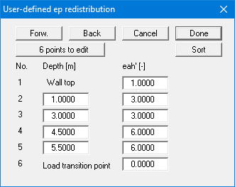
You can define several depths between the top of the wall and the transition point, to each of which you can appoint appropriate earth pressure ordinates. In subsequent computations, earth pressure will be redistributed in exactly the area defined by the polygon you have created. Using the example in the above dialog box the following diagram is obtained:

Figure 25 User-defined earth pressure redistribution
"Graph positioning preferences" menu item
If you are not happy with the automatic graph arrangement you can arrange them to suit your needs using this menu item. First, activate the "Manual graph positioning" radio button.
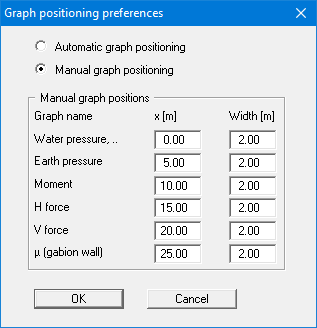
The graphs will then be shown at position "x" (central) with the specified "Width".
The fastest way to modify the position of a graph is to press the [F11] function key and then to pull the graph to the new position holding the left mouse button pressed.
"Graphics output preferences" menu item
Among other things, the screen graphics consist of several diagrams, presenting depth-oriented results. This menu item opens a dialog box which allows you to visualise the selected state variables on the screen by activating the corresponding check boxes.
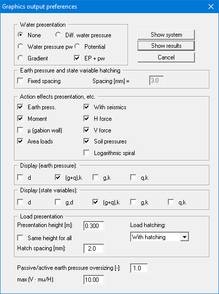
Overall, the dialog box is self-explanatory. For example, if the "Settlements" check box is activated, the stresses below the footing for the characteristic point are visualised. When "EP + pw" is selected, the sum of earth pressure and water pressure (pw) is displayed in the diagram for earth pressure.
When analysing using partial safety factors you will also see the group boxes "Display (earth pressure):", "Display (state variables):" and "Display (displacement):", in which you can activate display of the permanent (g) and/or live loads (q). In addition, the design values (d) can be displayed.
You can also specify hatching and the presentation height of loads. If the "Same height for all" check box is not selected, load visualisation is based on load size, the height of the presentation indicating the maximum load.
Leave the dialog box by pressing "Show system". If the system has already been analysed, you can leave the box by pressing "Show results" and then view the result graphics on the screen.
"Labelling preferences" menu item
This menu item allows you to specify labelling preferences for the system visualisation and the result graphics.
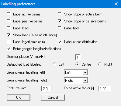
In the dialog box, you activate the required check boxes and select the preferences for alignment or font sizes. In addition, groundwater and berms labelling can be edited.
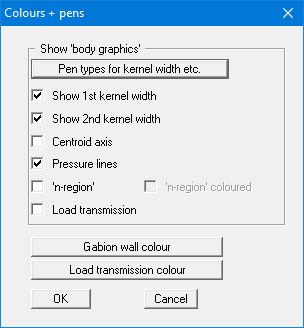
"Body pens + colours" menu item
The gabion body is visualised with a multitude of graphic elements (centroid axis, kernel width, etc.). Individual elements of the visualisation can be subdued, the pen types (dashed, dotted, etc.) and fill colours changed.
"Dimension lines" menu item
You can define a vertical and/or horizontal dimension line for the graphics in order to emphasise and clarify the system dimensions.
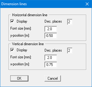
The distance to the gabion body is defined by means of the "y-position" for the horizontal dimension line and "x-position" for the vertical dimension line. Negative values define a position above or to the left of the gabion body. All values are in metres in the scale selected (see the menu item "Page size + margins/Manual resize (editor)" in section 8.8.3).
The fastest way to modify the position of the dimension line is to press the [F11] function key and then to pull the legend to the new position with the left mouse button pressed.
"Display system" menu item
Once a system has been analysed, all the state variables are automatically shown on screen. So as not to overburden the screen, certain elements of the system (for example, surcharges) are no longer shown. If you want to view all the system data without state variables, clicking this menu item will enable you to do so.
"Display results" menu item
After a system has been analysed, all state variables are automatically presented on the screen. If you used the menu item "System/Display system" to return to the system visualisation, you can go to this menu item to return to the result presentation without renewed analysis. Of course, this only works if the system has already been analysed.